
Effectiveness of Online Advertising
Causal Inference Experiments Case Study

Summary
Background
Star Digital, a large multichannel video service provider, spends a large portion of their budget on advertising. As the technological environment changed, so did Star Digital’s advertising strategy as they began to invest more heavily in online advertising such as banner ads. In order to get the most out of their budget, they actively evaluate the return on investment (RoI) of each ad medium. In evaluating the effectiveness of an online advertising campaign, Star Digital has designed a controlled experiment. Subjects were randomly assigned to a treatment group where they receive Star Digital ads or a control group where they receive ab ad for a charity on a selection of sites on an ad-serving software.
Business Question
Using the results of this experiment, Star Digital hopes to assess the causal effect of display advertising on sales conversion. In specific, there are three main questions they wish to address:
- Is online advertising effective for Star Digital?
- Is there a frequency effect of advertising on purchase?
- Which sites should Star Digital advertise on?
Analysis Performed
With regards to the first question, we performed a logistic regression to examine the influence of online advertising on purchases at Star Digital using test group as the regressor and conversion as the response. For the second question, we summed all impressions from the six sites and determined the impact of an increase in ad impressions on purchase via a logistic regression model adding total ad impressions as another regressor and its interaction. To address the last question, we defined an RoI metric in order to compare the effectiveness of sites 1 through 5 and site 6 and used logistic regression to estimate the effect of ad impressions from specific sites upon purchasing decision. We add replace total impressions with impressions from sites 1 to 5 and 6 and their interaction as regressors. We calculate RoI using our estimated causal impact per impression on purchase to determine the most profitable site decision for Star Digital.
Main Take-aways
A. We do not have enough evidence to conclude that online advertisement is effective for Star Digital if the number of impressions is not factored in. Whether customers are in the treatment or control group does not significantly affect the odds of purchase at Star Digital.
B. The total number of ad impressions online for consumers significantly influences whether they make a purchase with Star Digital or not. The odds of purchasing at Star Digital increase per ad impression seen for both the treatment and control group, but by a significantly bigger margin for those who saw Star Digital ads. This implies that users who are more active online are more likely to make a purchase in general and seeing Star Digital ads increases that probability moreover.
C. The total number of impressions from site 1 through 5 have significant effects on the purchasing decision regardless of test group while impressions from site 6 do not have a significant effect. However, each incremental impression on either sites 1 to 5 or site 6 increases the probability of purchasing significantly more for the group exposed to Star Digital ads than the control group.
D. Based on the ROI we recommend Star Digital invest its advertising budget into site 6 rather than sites 1-5.
More details in my github repo.
Sample Size Analysis
Now, we will discuss the implications of our sample size for the conclusions we can make. Because the sizes of the treatment and control groups are not even, we cannot use the same power test detailed in class as our sample violates the assumption that they are of equal size. Instead, we will use a test in the pwr package designed for unequal groups. 1 minus power refers to the probability of failing to detect an effect that exists. Therefore, a higher power reduces the probability that a real effect is undetected.
ptab2 = cbind(NULL, NULL)
for (i in c(.7, .75, .8, .85, .9, .95)){
  pwrt = pwr.t2n.test(n1 = 2656, n2 = 22647, sig.level = .05, power = i,
                      alternative = "two.sided")
  ptab2 = rbind(ptab2, cbind(pwrt$power, pwrt$d))
}

plot(ptab2[,1], ptab2[,2], type = "b", xlab = "Power", ylab = "Effect Size")
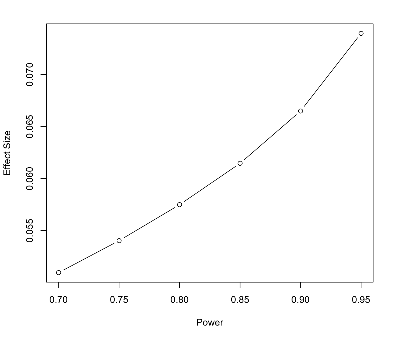
As we can see in the graph above, given our sample size and a standard significance level of 0.05, there is an increasing relationship between the level of power and the minimum effect size that can be reliably detected. In otherwords, at higher levels of power, there must be a larger effect to be detected reliable.
Randomization Check
Finally, we will perform t-tests to check if the randomization between the treatment and control groups was done sufficiently and that the groups are roughly homogenous outside of the treatment. If the groups are significantly different, the conclusions of our analyses may not be reliable.
t.test(imp_1 ~ test, data = star)
# Output of tests for sites 2 to 5 are hidden to reduce redundancy as results are
# similar to that of site 1 (sites 3/5 significant, sites 2/4 insignificant)
invisible(t.test(imp_2 ~ test, data = star))
invisible(t.test(imp_3 ~ test, data = star))
invisible(t.test(imp_4 ~ test, data = star))
invisible(t.test(imp_5 ~ test, data = star))
t.test(imp_6 ~ test, data = star)
t.test(sum1to5 ~ test, data = star)
Welch Two Sample t-test

data:  imp_1 by test
t = -3.905, df = 3574.1, p-value = 9.596e-05
alternative hypothesis: true difference in means is not equal to 0
95 percent confidence interval:
 -0.5961772 -0.1976257
sample estimates:
mean in group 0 mean in group 1
      0.5756777       0.9725791


	Welch Two Sample t-test

data:  imp_6 by test
t = 0.43156, df = 2898.4, p-value = 0.6661
alternative hypothesis: true difference in means is not equal to 0
95 percent confidence interval:
 -0.3176712  0.4969729
sample estimates:
mean in group 0 mean in group 1
       1.863705        1.774054


	Welch Two Sample t-test

data:  sum1to5 by test
t = -0.071371, df = 3268.6, p-value = 0.9431
alternative hypothesis: true difference in means is not equal to 0
95 percent confidence interval:
 -0.8402427  0.7812196
sample estimates:
mean in group 0 mean in group 1
       6.065512        6.095024
When we consider websites 1 to 5 on their own, there seems to be statistically significant difference between the treatment and control groups. This implies that the composition of people in the two groups are not necessarily homogenous. However, when it comes to the total number of impressions seen in sites 1 to 5, given their interchangeability and Star Digital’s inability to show adds on a specific site, there is not enough evidence to say that the groups are significantly different. Similarly, in terms of their impressions on site 6, there is not enough evidence to assert that the treatment and control groups are not homogenous.
Main Analysis
Now that we better understand the data we will be analyzing, we can move onto answering the three main questions that Star Digital has.
Question 1:
Is online advertising effective for Star Digital?
lm1 = glm(purchase ~ test, data = star, family = 'binomial')
summary(lm1)
exp(coef(lm1))
# This transformation of fitted model coefficients is done here and in further analyses
# so that they can be interpreted as the odds ratio.
Call:
glm(formula = purchase ~ test, family = "binomial", data = star)

Deviance Residuals:
   Min      1Q  Median      3Q     Max
-1.186  -1.186   1.169   1.169   1.202

Coefficients:
            Estimate Std. Error z value Pr(>|z|)
(Intercept) -0.05724    0.03882  -1.474   0.1404
test         0.07676    0.04104   1.871   0.0614 .
---
Signif. codes:  0 ‘***’ 0.001 ‘**’ 0.01 ‘*’ 0.05 ‘.’ 0.1 ‘ ’ 1

(Dispersion parameter for binomial family taken to be 1)

    Null deviance: 35077  on 25302  degrees of freedom
Residual deviance: 35073  on 25301  degrees of freedom
AIC: 35077

Number of Fisher Scoring iterations: 3

(Intercept)        test
  0.9443631   1.0797852
Interpretations
First, we will use logistic regression to determine whether being in the group that receives Star Digital ads has a significant increase in the odds of purchase. In the regression, the p-value for ‘test’ is 0.0614, which is greater than the acceptable significance level 0.05. This means there is not enough evidence to say whether the consumer is in the treatment or control group has an effect on whether he/she will eventually make a purchase at Star Digital. Hence, we do not have enough evidence to conclude that simply displaying online advertising is effective in stimulating purchases. Although we cannot confidently say that it is different from 0, we estimate that being part of the test group would increase the odds of purchasing Star Digital by 7.98%.
Question 2:
Is there a frequency effect of advertising on purchase? In particular, the question is whether increasing the frequency of advertising increases the probability of purchase?
star$total_imp = rowSums(star[,4:9])

lm2 = glm(purchase ~ test + total_imp + test*total_imp, data = star, family = 'binomial')
summary(lm2)
exp(coef(lm2))
Call:
glm(formula = purchase ~ test + total_imp + test * total_imp,
    family = "binomial", data = star)

Deviance Residuals:
    Min       1Q   Median       3Q      Max
-4.9145  -1.1266   0.1299   1.2156   1.2433

Coefficients:
                Estimate Std. Error z value Pr(>|z|)
(Intercept)    -0.169577   0.042895  -3.953 7.71e-05 ***
test           -0.013903   0.045613  -0.305    0.761
total_imp       0.015889   0.002876   5.524 3.32e-08 ***
test:total_imp  0.015466   0.003207   4.823 1.42e-06 ***
---
Signif. codes:  0 ‘***’ 0.001 ‘**’ 0.01 ‘*’ 0.05 ‘.’ 0.1 ‘ ’ 1

(Dispersion parameter for binomial family taken to be 1)

    Null deviance: 35077  on 25302  degrees of freedom
Residual deviance: 34190  on 25299  degrees of freedom
AIC: 34198

Number of Fisher Scoring iterations: 5

   (Intercept)           test      total_imp test:total_imp
     0.8440214      0.9861932      1.0160156      1.0155865
Interpretations
To answer this question, we first create a new variable summing all the impressions from the websites. Now, we need to determine the impact of ad frequency on purchase. Again, we will use logistic regression. Our results show that simply being subject to the Star Digital ads does not result in a significant increase in purchasing. This supports the conclusion we reached in Question 1.
Looking at the effect of total impressions on the odds of purchase, we see a very signifcant p-value, much lower than 0.05. This means that there is evidence that the total number of ad impressions for each consumer effects whether they make a purchase at Star Digital or not. The coefficent of the total impression term is 0.0159, which means that there is around a 1.6% increase in the odds of making purchasing at Star Digital for for each additional ad impression in the control group. This implies that more online activity increases the likelihood of purchasing from Star Digital, regardless of whether they are seeing Star Digital ads.
Now focusing on the treatment group, we again see p-value for the interaction between being in the treatment group and total impressions is well below than 0.05. This indicates a significant difference in the effect of an additional ad impression between the treatment and control group. Examining the coefficient on the interaction term, we see that above and beyond the 1.6% increase in purchase odds for the control group, consumers in the treatment group are expected to have an additional 1.5% increase in odds of purchasing from Star Digital for each ad impression.
As we can see, it appears that a higher frequency of advertising does increase the probability of purchase.
Question 3:
Which sites should Star Digital advertise on? In particular, should it put its advertising dollars in site 6 or in sites 1 through 5?
To address this question, we must first define a RoI metric in order to compare the effectiveness of sites 1 through 5 and site 6. To do so, we used the following formula as our criteria to assess the profitability of different sites:
ROI = ((Value of Purchase * Increase in Odds of Purchase) - Cost of Impression) / Cost of Impression
lm3 = glm(purchase ~ test + sum1to5 + imp_6 + test*sum1to5 + test*imp_6,
          data = star, family = 'binomial')
summary(lm3)
exp(coef(lm3))
Call:
glm(formula = purchase ~ test + sum1to5 + imp_6 + test * sum1to5 +
    test * imp_6, family = "binomial", data = star)

Deviance Residuals:
    Min       1Q   Median       3Q      Max
-5.1280  -1.1195   0.1185   1.2217   1.2472

Coefficients:
              Estimate Std. Error z value Pr(>|z|)
(Intercept)  -0.166556   0.042533  -3.916 9.01e-05 ***
test         -0.006087   0.045314  -0.134 0.893139
sum1to5       0.019452   0.003443   5.650 1.61e-08 ***
imp_6         0.003978   0.004294   0.927 0.354179
test:sum1to5  0.014617   0.003794   3.852 0.000117 ***
test:imp_6    0.013483   0.005405   2.494 0.012616 *
---
Signif. codes:  0 ‘***’ 0.001 ‘**’ 0.01 ‘*’ 0.05 ‘.’ 0.1 ‘ ’ 1

(Dispersion parameter for binomial family taken to be 1)

    Null deviance: 35077  on 25302  degrees of freedom
Residual deviance: 34166  on 25297  degrees of freedom
AIC: 34178

Number of Fisher Scoring iterations: 5

 (Intercept)         test      sum1to5        imp_6 test:sum1to5   test:imp_6
   0.8465755    0.9939313    1.0196422    1.0039860    1.0147240    1.0135741
Interpretations
Our final regression summary using logistic regression and assessing the effect of ads on certain websites again confirms our results from Question 1 that just being in the treatment or control group does not significantly affect the odds to purchase.
Additionally, the total impressions from site 1 through 5 has a significant effect on the odds of purchase purchase while there is not evidence to say that number of impressions from site 6 has a significant impact at the 95% confidence level. More specifically, we estimate that for each additional impression on sites 1 through 5, the odds of purchasing from Star Digital increases by 1.96%. However, each additional impression on site 6 leads to an expected increase in the odds of purchase by only 0.40%.
In addition, the p-value for interaction terms on being in the treatment group and the total number of impressions on each group of sites is very small and we have evidence to suggest that the treatment group’s purchase behavior changes differently with additional impressions than the treatment group. Compared to the control group, each additional impression from sites 1 to 5 for the treatment group is expected to have a 1.47% increase in purchase odds more than the 1.96% increase expected in the control group. Similarly, those in the treatment group are expected to have a 1.36% higher increase in odds of purchase for each additional site 6 ad than those in the control group.
Meanwhile, site 1 to 5 runs ads at 25 dollars per 1000 impressions whereas site 6 runs ads at 20 dollars per 1000 impressions. Therefore, our ROI is calculated as follows:
ROI_site1to5 = ((1200 * .0147240) - (25 / 1000)) / (25 / 1000)
ROI_site1to5
ROI_site6 = ((1200 * .0135741) - (20 / 1000)) / (20/1000)
ROI_site6
[1] 705.752
[1] 813.446
As we can see, there is a higher ROI in investing in ads on site 6 and we conclude that Star Digital should put its advertising dollars in site 6.
Concerns and Limitations
Now that our analysis is complete, we will briefly touch on some of the major threats and limitations of our results and conclusions.
Threats to Causal Inference
First, we will discuss the four key threats to causal inference and the extent to which they are present in this experiment.
-
Selection Bias: There appears to be a large threat of selection bias pressent in this experiment. Since the group of consumers participating in the experiment are not described, we do not know if they are representative of all potential customers that they would advertise to on these sites. In addition, the sample that is used for analysis is a choice-based sample with about one half of subjects resulting in purchases. Because of this design choice, we would need to do a transformation to map it back to the population in order to make proper inference and interpretations. Interpretations such as the increase in odds of purchase and RoI are likely skewed higher than they should be since the true conversion rate was 0.153% rather than the 50% represented in the sample.
-
Omitted Variable Bias: There are no demographic information of users is provided. For example, if variables such as gender or age is correlated to both the time spent on surfing websites and probability of subscribing the package, then those omitted bias will cause endogeneity of the experiment. Although using a randomized experiment should control for this, we do not have enough information to conclude whether randomization controlled for this. In addition, as we saw in our randomization checks, the treatment and control groups do show differences in activity on individual websites 1 through 5. Depending on the the content and nature of these websites, these differences in activity may reflect latent differences in the characteristics of the treatment and control group that may be correlated with the purchase decision.
-
Simultaneity Bias: It does not seem that simultaneity should be a threat to this as Star Digital assigned treatment and control and purchase decision should not determine the frequency of ads.
-
Measurement Error: The measurement method of impressions may be problematic to some extent as we don’t know the amount of time spent with the ad visible or if the user actually looked at the ad. Additionally, if ads that are hidden by software such as an ad blocker are still recorded, we may have inaccurate measurements.
Limitations
There are various other limitations in the experimental design that either hinder our conclusions or allow for more to be desired. First, it is unclear whether subject of the experiment are aware of the experiment. If they are, they may change their behavior or act in a way that they think is more desirable either socially or to the experimenter. Also, there may be some concern of interference as subjects could share information online which can undermine our ability to recover accurate causal estimates. Similarly, as this is the evaluation of a single ad campaign, users both in the treatment and control groups may have been inadvertently exposed to other Star Digital ads through either traditional media or a different online campaign during the experiment. Additionally, exposure to Star Digital advertisements could make people want to purchase the service in general, not only from Star Digital. It could make sense to use market share as another metric to examine. Finally, there is no information about conversion timing. If it’s a very long time, a conversion that occurred long after someone saw an ad may be counted as a view-through conversion although it’s not very plausible that the purchase actually stemmed from a banner ad seen long ago.
Key takeaways
Interpretation of interaction effect (secondary effect)
Interaction effect
Interaction term is an effect on effect, not effect of a variable on another variable.
Effect X(treatment) on Y: We believe that changing x by some amount, Y will change by some corresponding amount.
Interaction effect: We believe the causal relationship between X and Y depends on the magnitude of Z.


In this case, for question 2, we should use interaction effect even though the question is imbiguous to start with. I not only care about the effect of showing an advertising versus a charitable advertising on purchase, but also how does the strength of effect depends on how frequently I show you the advertising.
Interaction vs subsample analysis
What about we do a sub-sample regression? Just taking out the group that made purchase is somehow problematic.
Then problem with it is that it is not a causal problem. We don’t need an expriment to get the result if that’s what we care about because we don’t care what is a baseline conversion.
Think about the trick when business make people to buy fraudulent products.
“I have developed a magic pill to cure common cold. If you take a pill, your symptoms will be significantly released within a week and if you take extra, you will recover even faster.” – I am not telling you what would happen without the pill, you will still get better even without any pills in a week. The pill does nothing, and yet, you will see a frequency change.
In this case, maybe StarDigital ad is counterproductive, we will not see that if we don’t compare it with the baseline.
Baseline of treatment issue
What if we omit $\beta_1 X$ term?

In this case, if we omit the X term, for one, there will be omit variable problem for sure.
For two, it implies that we believe if we show zero advertising, the treatment effect of star digital ad equals zero, which is not a ridiculous hypothesis to make. But in practice, why make this assumption when we don’t have to.
General practice, run the full-fledged regression. Put in the isolated treatment term ($\beta_1 X$).
- If the baseline treatment effect is zero, $\beta_1$ will turn out to be zero or closed to zero (self contained) and insignificant and we will get what we want.
- However, if we omit it, in the alternative world where we do not omit it and $\beta_1$ is significant different from zero, we will be soooo wrong.
Logistic regression (Latent factor regression) coefficient
Converting coefficients of Log odds back to probability can be a hassle.
Log odds (actual dependent variable): log[P(purchase)/(1-P(purchase))]
Describing changes in odds, not probability: One unit change in X, leads to one unit change in log odds.
When we want to convert it back, we want a baseline conversion probability. In this particular case, we can get that conversion probability in the control group.

Marginal effect of logistic regression
Decreasing margin of effect?
We we observe the decreasing marginal effect from X on Y, means they don’t have linear relationship, then we might want to include X square term.