
Predicting Visitors for Restaurants
For suckers for Sashimi like me!

1. Project Definition & Introduction
When someone opens a restaurant, their focus is likely on making high-quality food that will make their customers happy. However, this does not cover all the problems they encounter. How do they effectively schedule the staff? How do they know the quantity of ingredients to order? If restaurants cannot solve these problems, their business will be hurt.
If restaurants can predict how many visitors will be in one day, it’s easier for them to make the arrangement. However, forecasting the number of visits is hard because it might be influenced by countless factors (eg weather, holiday, and location). It’s even harder for new restaurants with little historical data to make accurate predictions.
We are going to use reservation and visitation data to predict the total number of visitors to a restaurant for future dates. This information will help restaurants be more efficient and allow them to focus on creating an enjoyable dining experience for their customers.
Data Sources
The following information was taken straight from the Kaggle prompt:
Our data comes from two separate sites and can be downloaded from Kaggle:
Hot Pepper Gourmet (hpg): similar to Yelp, here users can search restaurants and also make a reservation onlineAirREGI / Restaurant Board (air): similar to Square, a reservation control and cash register system
We use historical visits, reservations, and store information from both sites to forecast the daily number of visitors for certain restaurants on given dates.
The training data covers the dates from 2016 until April 2017. The test set covers the last week of April and May of 2017. The test set is split based on time (the public fold coming first, the private fold following the public) and covers a chosen subset of the air restaurants.
Note that the test set intentionally spans a holiday week in Japan called the Golden Week.” Also there are days in both training and test set where the restaurant were closed and had no visitors. The training set omits days where the restaurants were closed, and in testing set, they are ignored in scoring.
File Descriptions
As mentioned above, there are datasets from two separate systems. Each file is prefaced with the source (eitherair or hpg) to indicate its origin. Each restaurant is associated with a unique air_store_id and hpg_store_id. Note that not all restaurants are covered by both systems, and that we have been provided data beyond restaurants for which we make predictions on. Latitudes and Longitudes are not exact to discourage de-identification of restaurants. (The file description details are from the website introduction)
- air_reserve.csv This file contains reservations made in the air system.
air_store_id- the restaurant’s id in the air systemvisit_datetime- the date and time of the visit for the reservationreserve_datetime- the date and time a reservation was madereserve_visitors- the number of visitors for that reservation
- hpg_reserve.csv This file contains reservations made in the hpg system.
hpg_store_id- the restaurant’s id in the hpg systemvisit_datetime- the date and time of visit for the reservationreserve_datetime- the date and time a reservation was madereserve_visitors- the number of visitors for that reservation
- air_store_info.csv This file contains stores information in the air system. Column names and contents are self-explanatory. Note the latitude and longitude are geographical information of the area to which the store belongs.
air_store_id, air_genre_name, air_area_name, latitude, longitude
4. hpg_store_info.csv This file contains stores information in the hpg system. Column names and contents are self-explanatory. Note: latitude and longitude are the latitude and longitude of the area to which the store belongs.
hpg_store_id
hpg_genre_name
hpg_area_name
latitude
longitude
-
store_id_relation.csv This file allows you to join select restaurants that have both the air and hpg system.
-
air_visit_data.csv This file contains historical visit data for the air restaurants.
air_store_idvisit_date- the datevisitors- the number of visitors to the restaurant on the date
- date_info.csv This file shows a submission in the correct format, including the days for which you must forecast.
calendar_dateday_of_weekholiday_flg- is the day a holiday in Japan
Model Summary
| Models Name | ERROR(RMSLE) |
|---|---|
| ARIMA | 0.56137 |
| PROPHET | 0.54208 |
| LIHGT GBM(LGBM) | 0.52412 |
| LSTM SEQ2SEQ | 0.50277 |
| LSTM + LGBM | 0.50002 |
We started by using ARIMA and PROPHET as our baseline model. Both are typical models when facing time-series related problem. However, the typical model can’t take external data we have into account such as weather and store location. We decided to use other models that are capable of overcoming these challenges.
We also decided to try some ensembling methods. Light GBM is a very popular model and also gives good performance. We also included LSTM which is another traditional model for time-series prediction. Finally, we got a RMSLE with 0.50002 with a combination of LSTM and LGBM.
Analysis Flow
We are following a very standard machine learning process which can be concluded as below chart:

Source: hackernoon
The first steps were to understand the main problem, get familiar with the structure of the data and decide what features we need. This is a Time-Series prediction, so we need to be careful about the sequence of the data. In any modeling process, the data that goes into a model plays a big role in ensuring accurate results. Therefore, the relevant features that helped achieve the objective were defined and an initial feature set was selected.
Following this, some noisy and missing data was removed. We had access to data on restaurant reservations, but the dataset was incomplete and not of much use to us. Thus we didn’t take this factor into account. Too many missing values might lead to a worse result even if it’s a good predictor.
Some fields’ values were imputed - for example, those of extreme actual visitor numbers on a specific day. After the data engineering, the core modeling process was started. Different algorithms were implemented on the feature set, along with cyclical addition and removal of features depending on performance and complexity of the features and the model used.
2. Feature Engineering
Because this is a time series problem, t’s better to take feature selection as the first step. Feature selection enables the machine learning algorithm to train faster. It reduces the complexity of a model and makes it easier to interpret and reduces the risk of overfitting. It also improves the accuracy of a model if the right subset is chosen.
Time Series Features
In order to take advantage of the date information, we extract year/month/day/weekday from the column visit_date as our features.
-
Visit date - original column in the data. The date visitor come to the restaurant. Used for mapping different data files
-
Day of week - day of the week. Use numeric value to represent. If the day is weekend, it might have more traffic than normal weekdays.
-
Month of the Year - different months also has different volume. This variable is kind of similar to season which showcase the seasonality of the time in a year
-
Holiday Status - whether a day is holiday. This vairable can indicate the holiday flag. If it’s holiday time, there might be higher traffic outside and restaurant might also have more number of visitors. Thus this shoud be a good predictor
-
Next day holiday - whether the next day is holiday. Days around holiday might also play a role in attracting visitors to restaurants. If the next day is holiday, people may be tried and don’t hand out in the previous
-
Previous day holiday - Same to the above two predictors
-
Consecutive Holidays - other than normal holiday flag data in the
data_info.csv, we believe consective holidays and the length of days off-work also have a say in restaurant visiting patterns. For example, if the holiday is Friday, we will mark Friday, and the followed weekend with 3. Same goes when Monday is holiday and so on. -
Seasons - Japan has four distinct seasons: March to May is spring; June to August is summer; September to November is autumn; and December to February is winter. Each season has very different temperatures and climates which might affect the traffic.
-
Prior Year Mapping One obvious solution to predicting visitors would be to look at how many customers came the year before. For example, if we are predicting for Jan 10, we might want to look at Jan 10th of the prior year. However, this is a slight problem here: what if Jan 10th of the previous year fell on a Saturday, but this year it falls on a Monday? To adjust this, we instead will take the number of visitors from the matching
week of the year& theday of the weektogether. After running our LightGBM model, this feature was in the top 5 in terms of importance.final['prev_visitors'] = final.groupby( [final['visit_date'].dt.week, final['visit_date'].dt.weekday])['visitors'].shift() -
Days since 25th (Paycheck Day. Yay!)
The next feature calculates how many days it has been since the previous 25th of the month. The 25th is special because this is when most Japanese people receive their monthly paycheck Japan Visa
In a country like the US, this may not play too large of a role as people simply use a credit card. In Japan, however, people seem to be averse to debt and prefer cash over credit cards (Business in Japan).
After running our LightGBM model, this feature was in the top 5 in terms of importance.
def daysToPrev25th(row):
    TARGET_DATE = 25
  if row['dayofmonth'] >= 25: 	return row['dayofmonth'] - TARGET_DATE
    else: 	return row['daysinPrevmonth'] - TARGET_DATE + row['dayofmonth']

air_visit["dayofmonth"] = air_visit["visit_date"].dt.day
air_visit["daysinPrevmonth"] = (air_visit["visit_date"] - pd.DateOffset(months=1)).dt.daysinmonth
air_visit["daysToPrev25th"] = air_visit.apply(lambda row:daysToPrev25th(row), axis=1)
Visit Features
Note that visitors does not exist in test set. Features such as locations and genres are categorical attributes and many missing values are involved. In this case, we need to create features on visitors , which will rely on the number of visitors to calculate. Therefore, we can feed visitors related features into our models to provide clues regarding stores.
Here, we calculate min, max, median, mean, and the number of times each store has been visited per each day of the week. The following code might look complicated but we are using the aggregate method of “group by” essentially.
def visitor_features(df, visitor_data):
    tmp = visitor_data.groupby(['air_store_id', 'dow'], as_index=False)['visitors'].min().rename(columns={'visitors': 'min_visitors'})
    df = pd.merge(df, tmp, how='left', on=['air_store_id', 'dow'])
visitor_data= train.copy()
train = visitor_features(train, visitor_data)
test = visitor_features(test, visitor_data)
- max visitors: maximum number of visitors for each store for a specific weekday
- min visitors: minimum number of visitors for each store for a specific weekday
- average visitors: average number of visitors for each store for a specific weekday
- count observations: number of observations for each store in a specific weekday. We take this feature into consideration because a number of stores don’t open to business everyday
- exponential moving average: the most recent data is weighted to have more of an impact
Geographical Features
Geographic features were not exactly straightforward to deal with. We had to do a bit of munging and pulling external data to determine the impact that locations had.
-
City - We weren’t provided with columns such as
region,city,neighorhood, etc. Instead, we had one column that included 5 levels of detail. Our dataset was in English, but the cities retained their original Japanese symbols. We had longitude and latitude data from 2 different systems to 6 decimal places, so the numbers sometimes did not match up exactly. So we need to split the column and select the information we need. -
Population and Density - To go along with this, we have also added the population for each of the cities. This information comes from both Simple Maps and verified with Wikipedia. This is the dataset that we combined with our training set. We made sure that every city was included and that there were no missing values. Population is in millions, population density is in thousands.
cities = ['Tokyo-to','Osaka-fu','Fukuoka-ken','Hyogo-ken', 'Hokkaido','Hiroshima-ken','Shizuoka-ken', 'Miyagi-ken','Niigata-ken','Osaka','Kanagawa-ken', 'Saitama-ken'] population = [2.7, 1.2, 8.6, 1.1, 1.0, 1.2, 1.5,3.7, 1.5, .8, 2.6, 1.6] density = [11.9, 5.4, 13.9, 1.3, 1.3, 1.7, .5, 8.5,2.7, .7, 11.9, 4.4] pop = pd.DataFrame(list(zip(cities, population, density)), columns=['cities','population', 'density']) -
Restaurant Types - this information contains which food type the restaurant is selling. We are provided with restaurant types for every store in our data, but the labels are not consistent. In order to gain more meaningful data from the types of restaurants we are provided, we convert the many specific labels into more general labels that capture the restaurant type. After looking at the plot below, we are doubtful that restaurant type plays much of a role for the restaurants we are predicting. It doesn’t really seem like there is much of a relationship between restaurant type and expected visitors.
# Quick example
all_stores['Food_Type'] = np.where(all_stores['Food_Type']
     .str.contains(('Izakaya'),'Izakaya',all_stores['Food_Type'])
Data Cleaning
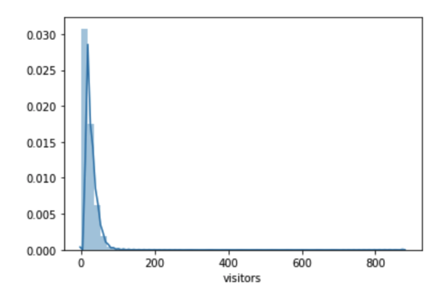
Outliers
As we can see, the number of visitors is highly left skewed and the max number reached 877 which seems unreasonable. These values might be outliers.
We simply define outliers using the following rules:
- Data point that falls outside of 1.5 times of an interquartile range above the 3rd quartile and below the 1st quartile
- Data point that falls outside of 3 standard deviations.
q1, q3= np.percentile(train.visitors,[25,75])
iqr = q3 - q1
lower_bound = q1 -(1.5 * iqr)
upper_bound = q3 +(1.5 * iqr)
train.loc[train.visitors > upper_bound ,'visitors'] = upper_bound
train.loc[train.visitors < lower_bound ,'visitors'] = lower_bound
After this process we will get a nicer distribution.

3. Modeling
Given the Time Series nature of our prediction exercise, we started by implementing the model ARIMA, short for Auto Regressive Integrated Moving Average, which is a model that explains a given time series based on its own past values, i.e. its own lags and the lagged forecast errors, so that equation can be used to forecast future values. But as we can see from this explanation, ARIMA model doesn’t take into consideration external factors to forecast the number of visitors.
We then implemented another famous model for Time series which is Facebook Prophet, which is a procedure based on an additive model where non-linear trends are fit with yearly, weekly, and daily seasonality, plus holiday effects. However, this model works best with time series that have strong seasonal effects and several seasons of historical data, which is not the case in our prediction exercise.
That’s when we shifted our approach to Light GBM, which is a gradient boosting framework that uses tree based learning algorithms. The advantage of this approach is that it doesn’t need any statistical assumptions in the backend. Besides, it determines which features have the highest discriminative powers, which enables us to give valuable insights to the restaurant owners.
ARIMA
# forecasting - register cores for parallel processing
registerDoMC(detectCores()-1)
fcst_matrix <- foreach(i=1:nrow(train_ts),.combine=rbind, .packages=c("forecast")) %dopar% {
    fcst_ets <- forecast(ets(train_ts[i,]),h=fcst_intv)$mean
    fcst_nnet <- forecast(nnetar(train_ts[i,]),h=fcst_intv)$mean
    fcst_arima <- forecast(auto.arima(train_ts[i,]),h=fcst_intv)$mean
    fcst_ses <- forecast(HoltWinters(train_ts[i,], beta=FALSE, gamma=FALSE),h=fcst_intv)$mean
    fcst_matrix <- rbind(fcst_ets, fcst_nnet, fcst_arima, fcst_ses)
}

# post-processing the forecast table
fcst_matrix_mix <- aggregate(fcst_matrix,list(rep(1:(nrow(fcst_matrix)/4),each=4)),mean)[-1]
fcst_matrix_mix[fcst_matrix_mix < 0] <- 0
colnames(fcst_matrix_mix) <- as.character(
  seq(from = as.Date("2017-04-23"), to = as.Date("2017-05-31"), by = 'day'))
fcst_df <- as.data.frame(cbind(train_wide[, 1], fcst_matrix_mix))
colnames(fcst_df)[1] <- "air_store_id"

# melt the forecast data frame from wide to long format for final submission
fcst_df_long <- melt(
  fcst_df, id = 'air_store_id', variable.name = "fcst_date", value.name = 'visitors')
fcst_df_long$air_store_id <- as.character(fcst_df_long$air_store_id)
fcst_df_long$fcst_date <- as.Date(parse_date_time(fcst_df_long$fcst_date,'%y-%m-%d'))
fcst_df_long$visitors <- as.numeric(fcst_df_long$visitors)
Prophet
# Prediction
from fbprophet import Prophet
# This is used for suppressing prophet info messages.
import logging
logging.getLogger('fbprophet.forecaster').propagate = False

number_of_stores = test['store_id'].nunique()
date_range = pd.date_range(start=pd.to_datetime('2016-07-01'),
                           end=pd.to_datetime('2017-04-22'))
forecast_days = (pd.to_datetime('2017-05-31')- pd.to_datetime('2017-04-22')).days

for cnt, store_id in enumerate(test['store_id'].unique()):
    print('Predicting %d of %d.'%(cnt, number_of_stores), end='\r')
    data = visitor_data[visitor_data['air_store_id'] == store_id]
    data = data[['visit_date', 'visitors']].set_index('visit_date')
    # Ensure we have full range of dates.
    data = data.reindex(date_range).fillna(0).reset_index()
    data.columns = ['ds', 'y']

    m = Prophet(holidays=df_holidays)
    m.fit(data)
    future = m.make_future_dataframe(forecast_days)
    forecast = m.predict(future)
    forecast = forecast[['ds', 'yhat']]
    forecast.columns = ['id', 'visitors']
    forecast['id'] = forecast['id'].apply(lambda x:'%s_%s'%(store_id, x.strftime('%Y-%m-%d')))
    forecast = forecast.set_index('id')
    test.update(forecast)
print('\n\nDone.')
LightGBM
#import lightgbm as lgbm
from sklearn import metrics
from sklearn import model_selection

np.random.seed(42)

model = lgbm.LGBMRegressor(
    objective='regression',
    max_depth=5,
    num_leaves=5 ** 2 - 1,
    learning_rate=0.007,
    n_estimators=30000,
    min_child_samples=80,
    subsample=0.8,
    colsample_bytree=1,
    reg_alpha=0,
    reg_lambda=0,
    random_state=np.random.randint(10e6)
)

folds = 6
cv = model_selection.KFold(n_splits= folds, shuffle=True, random_state=42)

val = [0] * folds

sub = submission['id'].to_frame()
sub['visitors'] = 0

feature_importances = pd.DataFrame(index=train_x.columns)

for i, (fit_idx, val_idx) in enumerate(cv.split(train_x, train_y)):

    X_fit = train_x.iloc[fit_idx]
    y_fit = train_y.iloc[fit_idx]
    X_val = train_x.iloc[val_idx]
    y_val = train_y.iloc[val_idx]

    model.fit(
        X_fit,
        y_fit,
        eval_set=[(X_fit, y_fit), (X_val, y_val)],
        eval_names=('fit', 'val'),
        eval_metric='l2',
        early_stopping_rounds=200,
        feature_name=X_fit.columns.tolist(),
        verbose=False
    )

    val[i] = np.sqrt(model.best_score_['val']['l2'])
    sub['visitors'] += model.predict(test_x, num_iteration=model.best_iteration_)
    feature_importances[i] = model.feature_importances_

    print('Fold {} RMSLE: {:.5f}'.format(i+1, val_scores[i]))

sub['visitors'] /= n_splits
sub['visitors'] = np.expm1(sub['visitors'])

val_mean = np.mean(val_scores)
val_std = np.std(val_scores)

print('Local RMSLE: {:.5f} (±{:.5f})'.format(val_mean, val_std))
LSTM seq2seq + Encoder/Decoder
Note that we have included all of the details below for this model in particular because this is our final model. Additionally, this model is best suited for this problem.
Motivation
LSTM is a great solution for relatively short sequences, up to 100-300 items. On longer sequences LSTM still works, but can gradually forget information from the oldest items. In our dataset, the timeseries is up to 478 days long, so we decided to implement encoder and decoder to “strengthen” LSTM memory.
We are using the encoder and decoder structure in the Sequence-to-sequence learning (Seq2Seq) concept, which is about training models to convert sequences from one domain (e.g. sentences in English) to sequences in another domain (e.g. the same sentences translated to French).
We used one LSTM RNN layer as “encoder": it processes the input sequence and returns its own internal state. Note that we discard the outputs of the encoder RNN, only recovering the state. This state will serve as the “context”, or “conditioning”, of the decoder in the next step.
And then we used another RNN layer with 2 hidden LSTM model acts as “decoder": it is trained to predict the next characters of the target sequence, given previous characters of the target sequence. Specifically, it is trained to turn the target sequences into the same sequences but offset by one timestep in the future, a training process called “teacher forcing” in this context. Importantly, the encoder uses as initial state the state vectors from the encoder, which is how the decoder obtains information about what it is supposed to generate.
Data Preparation
1) Basic tidying of the training and test table
# Drop unnecessary columns
train_df = train_df.drop(columns=[ 'population', 'reserve_visitors', 'days_diff', 'day', 'season'])
test = test.drop(columns=['population', 'reserve_visitors','days_diff', 'day', 'season'])
# Refine column names
train_df = train_df.rename({'visitors_x': 'visitors'}, axis = 1)
train_df = train_df.rename({'day_of_week_y': 'day_of_week'}, axis = 1)
train_df = train_df.rename({'month_y': 'month'}, axis = 1)
train_df = train_df.rename({'longitude_y': 'longitude'}, axis = 1)
train_df = train_df.rename({'latitude_y': 'latitude'}, axis = 1)
test = test.rename({'latitude_y': 'latitude'}, axis = 1)
test = test.rename({'longitude_y': 'longitude'}, axis = 1)
test = test.rename({'month_y': 'month'}, axis = 1)
test = test.rename({'day_of_week_y': 'day_of_week'}, axis = 1)
# Clean unnecessary columns
train_df = train_df.loc[:, ~train_df.columns.str.contains('^Unnamed')]
test = test.loc[:, ~test.columns.str.contains('^Unnamed')]
# Fill the cells of missing values with -1
train_df = train_df.fillna(-1)
test = test.fillna(-1)
2) Encode categorical columns
There are several categorical columns in the dataset, which are ‘Food_Type’, ‘day_of_week’, ‘air_store_id’ that needs to be transferred. One-hot encoding may provide better result, but we applied labels encoding to avoid high dimensional feature space.
# Weekday
le_weekday = LabelEncoder()
le_weekday.fit(train_df['day_of_week'])
train_df['day_of_week'] = le_weekday.transform(train_df['day_of_week'])
test['day_of_week'] = le_weekday.transform(test['day_of_week'])

# id
le_id = LabelEncoder()
le_id.fit(train_df['air_store_id'])
train_df['air_store_id'] = le_id.transform(train_df['air_store_id'])
test['air_store_id'] = le_id.transform(test['air_store_id'])

# food type
le_ftype = LabelEncoder()
le_ftype.fit(train_df['Food_Type'])
train_df['Food_Type'] = le_ftype.transform(train_df['Food_Type'])
test['Food_Type'] = le_ftype.transform(test['Food_Type'])
3) Simultaneous transformation of Train and test sets
Considering the input data structure the LSTM RNN model needed, we filled up all the dates within the whole time span (2016-01-01 ~ 2017-05-31) for each stores with number of visitors as 0 on those dates, and the time-independent features (food types, longitude, latitude, etc) are “stretched” to timeseries length.
# combine train and test sets
X_all = train_df.append(test)
# date table (includes all dates for training and test period)
dates = np.arange(np.datetime64(X_all.visit_date.min()),
                  np.datetime64(X_all.visit_date.max()) + 1,
                  datetime.timedelta(days=1))
ids = X_all['air_store_id'].unique()
dates_all = dates.tolist()*len(ids)
ids_all = np.repeat(ids, len(dates.tolist())).tolist()
df_all = pd.DataFrame({"air_store_id": ids_all, "visit_date": dates_all})
df_all['visit_date'] = df_all['visit_date'].copy().apply(lambda x: str(x)[:10])

# create copy of X_all with data relevant to 'visit_date'
X_dates = X_all[['visit_date', 'year','month','week',\
                 'is_holiday','next_day','prev_day',\
                 'daysToPrev25th','day_of_week','Consecutive_holidays']].copy()

# remove duplicates to avoid memory issues
X_dates = X_dates.drop_duplicates('visit_date')

# merge dataframe that represents all dates per each restaurant with information about each date
df_to_reshape = df_all.merge(X_dates,
                             how = "left",
                             left_on = 'visit_date',
                             right_on = 'visit_date')

# create copy of X_all with data relevant to 'air_store_id'
X_stores = X_all[['air_store_id', 'Food_Type', 'latitude','longitude']].copy()

# remove duplicates to avoid memory issues
X_stores = X_stores.drop_duplicates('air_store_id')

# merge dataframe that represents all dates per each restaurant with information about each restaurant
df_to_reshape = df_to_reshape.merge(X_stores,
                                    how = "left",
                                    left_on = 'air_store_id',
                                    right_on = 'air_store_id')
# merge dataframe that represents all dates per each restaurant with inf. about each restaurant per specific date
df_to_reshape = df_to_reshape.merge(X_all[['air_store_id', 'visit_date',\
                                           'prev_visitors', 'mean_visitors',\
                                       'median_visitors', 'max_visitors', \
                                           'min_visitors','count_observations'\
                                           ,'visitors']],
                                    how = "left",
                                    left_on = ['air_store_id', 'visit_date'],
                                    right_on = ['air_store_id', 'visit_date'])

# separate 'visitors' into output array
Y_lstm_df = df_to_reshape[['visit_date', 'air_store_id', 'visitors']].copy().fillna(0)

# take log(y+1)
Y_lstm_df['visitors'] = np.log1p(Y_lstm_df['visitors'].values)

# add flag for days when a restaurant was closed
df_to_reshape['closed_flag'] = np.where(df_to_reshape['visitors'].isnull() &
                                        df_to_reshape['visit_date'].isin(train_df['visit_date']).values,1,0)

# drop 'visitors' and from dataset
df_to_reshape = df_to_reshape.drop(['visitors'], axis = 1)

# fill in NaN values
df_to_reshape = df_to_reshape.fillna(-1)

# list of df_to_reshape columns without 'air_store_id' and 'visit_date'
columns_list = [x for x in list(df_to_reshape.iloc[:,2:])]
4) Normalize all numerical values
We bounded all numerical values between -1 and 1. To avoid data leakage ‘fit’ should be made on train data and ‘transform’ on train and test data in this case all data in test set is taken from train set, thus fit/transform on all data.
scaler = MinMaxScaler(feature_range=(-1, 1))
scaler.fit(df_to_reshape[columns_list])
df_to_reshape[columns_list] = scaler.transform(df_to_reshape[columns_list])
5) Reshape data structure for Neural Network and Encoder/Decoder
# reshape X into (samples, timesteps, features)
X_all_lstm = df_to_reshape.values[:,2:].reshape(len(ids),
                                                len(dates),
                                                df_to_reshape.shape[1]-2)

# isolate output for train set and reshape it for time series
Y_lstm_df = Y_lstm_df.loc[Y_lstm_df['visit_date'].isin(train_df['visit_date'].values) &
                          Y_lstm_df['air_store_id'].isin(train_df['air_store_id'].values),]
Y_lstm = Y_lstm_df.values[:,2].reshape(len(train_df['air_store_id'].unique()),
                                       len(train_df['visit_date'].unique()),
                                       1)
# test dates
n_test_dates = len(test['visit_date'].unique())
6) Training and validation split
There are two ways to split timeseries into training and validation datasets:
- Walk-forward split. This is not actually a split: we train on full dataset and validate on full dataset, using different timeframes. Timeframe for validation is shifted forward by one prediction interval relative to timeframe for training.
- Side-by-side split. This is traditional split model for mainstream machine learning. Dataset splits into independent parts, one part used strictly for training and another part used strictly for validation.
Walk-forward is preferable, because it directly relates to the competition goal: predict future values using historical values. But this split consumes data points at the end of timeseries, thus making hard to train model to precisely predict the future.
We used validation (with walk-forward split) only for model tuning. Final model to predict future values was trained in blind mode, without any validation.
# make additional features for number of visitors in t-1, t-2, ... t-7
t_minus = np.ones([Y_lstm.shape[0],Y_lstm.shape[1],1])
for i in range(1,8):
    temp = Y_lstm.copy()
    temp[:,i:,:] = Y_lstm[:,0:-i,:].copy()
    t_minus = np.concatenate((t_minus[...], temp[...]), axis = 2)
t_minus = t_minus[:,:,1:]
print ("t_minus shape", t_minus.shape)

# split X_all into training and test data
X_lstm = X_all_lstm[:,:-n_test_dates,:]
X_lstm_test = X_all_lstm[:,-n_test_dates:,:]

# add t-1, t-2 ... t-7 visitors to feature vector
X_lstm = np.concatenate((X_lstm[...], t_minus[...]), axis = 2)

# split training set into train and validation sets
X_tr = X_lstm[:,39:-140,:]
Y_tr = Y_lstm[:,39:-140,:]

X_val = X_lstm[:,-140:,:]
Y_val = Y_lstm[:,-140:,:]
Model
1) Model Structure Building
The encoder takes input features of 39 days (t1, t2 … t39) and encode their hidden states through LSTM neural network. Then it pass the hidden states to decoder. Decoder use them with the features of 39 days shifted 1 day forward (t2, t3 … T40) to predict number of visitors per each of 829 restaurants in t_40.
Methods used to address overfitting: we applied dropout and recurrent dropout regularization in all RNN layers and adjust the epoch size to prevent overfitting.
# MODEL FOR ENCODER AND DECODER -------------------------------------------
num_encoder_tokens = X_lstm.shape[2]
latent_dim = 256

# encoder training
encoder_inputs = Input(shape = (None, num_encoder_tokens))
encoder = LSTM(latent_dim,
               batch_input_shape = (1, None, num_encoder_tokens),
               stateful = False,
               return_sequences = True,
               return_state = True,
               recurrent_initializer = 'glorot_uniform')

encoder_outputs, state_h, state_c = encoder(encoder_inputs)
encoder_states = [state_h, state_c] # 'encoder_outputs' are ignored and only states are kept.

# Decoder training, using 'encoder_states' as initial state.
decoder_inputs = Input(shape=(None, num_encoder_tokens))

decoder_lstm_1 = LSTM(latent_dim,
                      batch_input_shape = (1, None, num_encoder_tokens),
                      stateful = False,
                      return_sequences = True,
                      return_state = False,
                      dropout = 0.4,
                      recurrent_dropout = 0.4) # True

decoder_lstm_2 = LSTM(128,
                     stateful = False,
                     return_sequences = True,
                     return_state = True,
                     dropout = 0.4,
                     recurrent_dropout = 0.4)

decoder_outputs, _, _ = decoder_lstm_2(decoder_lstm_1(decoder_inputs, initial_state = encoder_states))
decoder_dense = TimeDistributed(Dense(Y_lstm.shape[2], activation = 'relu'))
decoder_outputs = decoder_dense(decoder_outputs)

# training model
training_model = Model([encoder_inputs, decoder_inputs], decoder_outputs)
training_model.compile(optimizer = 'adam', loss = 'mean_squared_error')

# GENERATOR APPLIED TO FEED ENCODER AND DECODER ---------------------------
# generator that randomly creates times series of 39 consecutive days
# theses time series has following 3d shape: 829 restaurants * 39 days * num_features
def dec_enc_n_days_gen(X_3d, Y_3d, length):
    while 1:
        decoder_boundary = X_3d.shape[1] - length - 1

        encoder_start = np.random.randint(0, decoder_boundary)
        encoder_end = encoder_start + length

        decoder_start = encoder_start + 1
        decoder_end = encoder_end + 1

        X_to_conc = X_3d[:, encoder_start:encoder_end, :]
        Y_to_conc = Y_3d[:, encoder_start:encoder_end, :]
        X_to_decode = X_3d[:, decoder_start:decoder_end, :]
        Y_decoder = Y_3d[:, decoder_start:decoder_end, :]

        yield([X_to_conc,
               X_to_decode],
               Y_decoder)
2) Generator applied to feed encoder and decoder
Our generator that randomly creates times series of 39 consecutive days. And those time series has following 3-D shape: 829 restaurants * 39 days * num_features.
def dec_enc_n_days_gen(X_3d, Y_3d, length):
    while 1:
        decoder_boundary = X_3d.shape[1] - length - 1

        encoder_start = np.random.randint(0, decoder_boundary)
        encoder_end = encoder_start + length

        decoder_start = encoder_start + 1
        decoder_end = encoder_end + 1

        X_to_conc = X_3d[:, encoder_start:encoder_end, :]
        Y_to_conc = Y_3d[:, encoder_start:encoder_end, :]
        X_to_decode = X_3d[:, decoder_start:decoder_end, :]
        Y_decoder = Y_3d[:, decoder_start:decoder_end, :]

        yield([X_to_conc,
               X_to_decode],
               Y_decoder)
3) Training the model
Training on X_tr/Y_tr and validate with X_val/Y_val. To perform validation training on validation data should be made instead of training on full data set. Then validation check is made on period outside of training data
'''
training_model.fit_generator(dec_enc_n_days_gen(X_tr, Y_tr, 39),
                             validation_data = dec_enc_n_days_gen(X_val, Y_val, 39),
                             steps_per_epoch = X_lstm.shape[0],
                             validation_steps = X_val.shape[0],
                             verbose = 1,
                             epochs = 1)
'''

# Training on full dataset
training_model.fit_generator(dec_enc_n_days_gen(X_lstm[:,:,:], Y_lstm[:,:,:], 39),
                            steps_per_epoch = X_lstm[:,:,:].shape[0],
                            verbose = 1,
                            epochs = 5)
4) Perform Prediction
The function takes 39 days before first prediction day (input_seq), then using encoder to identify hidden states for these 39 days. Next, decoder takes hidden states provided by encoder, and predicts number of visitors from day 2 to day 40. Day 40 is the first day of target_seq.
Predicted value for day 40 is appended to features of day 41. Then function takes period from day 2 to day 40 and repeat the process unil all days in target sequence get their predictions.
The output of the function is the vector with predictions that has following shape: 820 restaurants * 39 days * 1 predicted visitors amount
def predict_sequence(inf_enc, inf_dec, input_seq, Y_input_seq, target_seq):
    # state of input sequence produced by encoder
    state = inf_enc.predict(input_seq)

    # restrict target sequence to the same shape as X_lstm_test
    target_seq = target_seq[:,:, :X_lstm_test.shape[2]]


    # create vector that contains y for previous 7 days
    t_minus_seq = np.concatenate((Y_input_seq[:,-1:,:], input_seq[:,-1:, X_lstm_test.shape[2]:-1]), axis = 2)

    # current sequence that is going to be modified each iteration of the prediction loop
    current_seq = input_seq.copy()


    # predicting outputs
    output = np.ones([target_seq.shape[0],1,1])
    for i in range(target_seq.shape[1]):
        # add visitors for previous 7 days into features of a new day
        new_day_features = np.concatenate((target_seq[:,i:i+1,:], t_minus_seq[...]), axis = 2)

        # move prediction window one day forward
        current_seq = np.concatenate((current_seq[:,1:,:], new_day_features[:,]), axis = 1)


        # predict visitors amount
        pred = inf_dec.predict([current_seq] + state)

        # update t_minus_seq
        t_minus_seq = np.concatenate((pred[:,-1:,:], t_minus_seq[...]), axis = 2)
        t_minus_seq = t_minus_seq[:,:,:-1]

        # update predicitons list
        output = np.concatenate((output[...], pred[:,-1:,:]), axis = 1)

        # update state
        state = inf_enc.predict(current_seq)

    return output[:,1:,:]

# inference encoder
encoder_model = Model(encoder_inputs, encoder_states)

# inference decoder
decoder_state_input_h = Input(shape=(latent_dim,))
decoder_state_input_c = Input(shape=(latent_dim,))
decoder_states_inputs = [decoder_state_input_h, decoder_state_input_c]
decoder_outputs,_,_ = decoder_lstm_2(decoder_lstm_1(decoder_inputs,
                                                    initial_state = decoder_states_inputs))
decoder_outputs = decoder_dense(decoder_outputs)
decoder_model = Model([decoder_inputs] + decoder_states_inputs,
                      [decoder_outputs])

# Predicting test values
enc_dec_pred = predict_sequence(encoder_model,
                                decoder_model,
                                X_lstm[:,-X_lstm_test.shape[1]:,:],
                                Y_lstm[:,-X_lstm_test.shape[1]:,:],
                                X_lstm_test[:,:,:])
Evaluation
Finally, we aggregated the prediction of both LGBM and seq2seq, which enabled us to get the best evaluation metric:
| Models Name | ERROR(RMSLE) |
|---|---|
| ARIMA. | 0.56137 |
| PROPHET | 0.54208 |
| LIHGT GBM(LGBM) | 0.52412 |
| LSTM SEQ2SEQ | 0.50277 |
| LSTM + LGBM | 0.50002 |
The metric used to evaluate our model is RMSLE (root mean squared logarithmic error) $$ \sqrt{\frac{1}{n} \sum_{i=1}^n (\log(p_i + 1) - \log(a_i+1))^2 } $$ where:
n is the total number of observations p_i is the prediction of visitors a_i is the actual number of visitors
We chose this metric for the following reasons:
- First, we care about percentage errors more than the absolute value of errors.
- Second, we want to penalize under estimating the number of visitors more than overestimating it, because underestimating will lead to a bad customer experience which is our top priority.
4. Business Insight
Normally we would provide recommendations in this section. Because we are only looking to sell our system in this project, we are instead providing reasons for why someone should buy our product.
We are looking to persuade a restaurant owner to purchase our product. For them, the decision ultimately comes down to: “How much will these predictions actually help me out? I believe I know the business and have good intuition about how many people will come to the restaurant. Are their predictions any better than me? How much money will they save for me?”
To quantify this, we decided to run a couple of simulations on our training data based on intuition to see how good our results would be. For reference, our daily percent error (using MAPE) was 50%.
-
Using the previous day, the manager would be off by 113% on average.
-
Using the same weekday from the previous week, the manager would be off by 94% on average.
# One day
df['prev_day_visitors'] = df['visitors_x'].shift(1)
df = df.groupby('air_store_id').apply(lambda group: group.iloc[1:, ])
# One week
df['prev_week_visitors'] = df.groupby([df['visit_date'].dt.weekday])['visitors_x'].shift()
df.groupby('air_store_id').apply(lambda group: group.iloc[7:, ])
# Error
df['difference_decimal'] = abs(
    df['visitors_x'] - df['prev_day_visitors']) / df['visitors_x']
Staffing
The hourly minimum wage in Japan translates to roughly $8.30 USD. Overstaffing by 2 people for a given 8-hour day equates to roughly $130 in unnecessary expenses. On the flip side, understaffing means a poor customer experience as wait time is longer. We believe this provides strong support for the purchase of our system.
Supply Chain
Although we are not able to quantify the supply chain as easily as we can with staffing costs, owners are able to reduce expenses if they have a more accurate picture of how many customers they expect to see. Purchasing too much leads to waste, and purchasing too little means running out of ingredients and making your customers upset. Using our system provides a more stable data-driven approach to this problem.
Smoothing Demand
Although not covered in our project, an individual will be able to look at their past data and gain an unbiased view of seasonality that occurs throughout the year. If they are looking for stability week-by-week or month-by-month to even out their supply purchases or keep the correct number of people on board, they can use their past data to aid in offering of incentives to drive customers where they see fit.
Important Features
Another insight we can provide the manager is an understanding of the most important features that drives their business. In particular, we found the following 5 to be most important when we ran our LightGBM model:
(1) Previous year mapping
(2) Days since previous 25th
(3) Holiday flag
(4) Aggregated visitors per day of week
(5) Exponential Moving Average
5. Limitations & Next Steps
To address the limitations of our predictive models, we could focus on the following dimensions to improve model performance.
Feature Improvement
We could pay more attention to feature engineering. We could include weather data in our model since the weather condition is likely to affect restaurant traffic. In addition, the distance of a restaurant to the busiest area might also contribute to the prediction of visiting frequency. Restaurants in busy areas are likely to have more traffic than those in suburb areas. We could also improve upon the feature selection process. The light GBM method provides the importance of each feature. Using this information, we are able to either remove unimportant features or add additional features that are similar to important features.
Expand the Timespan
Our current model is trained on data of 2-year time period. If we are able to collect data of longer time span and train our model on the enriched dataset, our model might be able to generate more accurate predictions.

References
https://blog.keras.io/a-ten-minute-introduction-to-sequence-to-sequence-learning-in-keras.html https://github.com/Arturus/kaggle-web-traffic https://github.com/MaxHalford/kaggle-recruit-restaurant/blob/master/Solution.ipynb https://www.kaggle.com/pureheart/1st-place-lgb-model-public-0-470-private-0-502 https://www.kaggle.com/plantsgo/solution-public-0-471-private-0-505 https://www.kaggle.com/h4211819/holiday-trick https://www.kaggle.com/c/recruit-restaurant-visitor-forecasting/discussion/49100